Grid Refinement
Introduction
The grid refinement code was developed to allow for localized refinement of a grid. The idea itself came from my work with MODFLOW USG, which allowed for local refinement of model grids using a quad tree refinement method. I wanted to develop a method within R that could allow me to quickly refine a grid, and then use that grid for any analysis I wanted to perform. What follows is an explanation of the code, assumptions, and examples of a grid refinement method in R. For those who wish to jump into exploring and playing with the code right away, there is a shiny app in which you can do just that here GridRefinement App, and the code for the shiny app is located here ShinyAppCode. As for my motivation for developing this, I wanted a method that was fairly easy and fast to use, produced a simple tabular dataset that could easily be applied to different applications, and a method that relied on the data to produce the grid and not the user defining the grid. The first objective is fairly obvious but I wanted a single function that I could feed point locations, along with some basic grid information, and produce a grid dataset from. Which leads to the second objective of having a simple table output that contains all the information need to graphically produce the grid or use it for any type of analysis. The idea is that making the output simple will allow for it to easily be used or converted into necessary data types for further analysis or use. I plan to expand on this point further with examples in the future with a different post. The last objective was to let the data define the grid and not the user. This desire came from my work with spatial data. Many times I would work with spatial data that is located in a projected coordinate system and would have to produce a grid around the data or area of interest in order to perform some spatial analysis (IDW, Kriging, etc.). I would start with always defining the origin and cell size and overlying a grid over the data. That required that I do some preliminary analysis before hand, and usually some trail and error to get a grid that would work. This method simply requires the point locations and handles the rest, as usually the origin was not important for the actual work. I just needed a grid centered around the data.
Code
The code itself is located on github and consists of four functions. The four functions are:
- Make Grid
- Ghost Nodes
- Quad Tree
- Grid Refinement
The first three functions are used in the final function “Grid Refinement” to produce the final function to produce the grid. For each function I will describe the general code and how it works along with examples to show the step by step process of producing the final grid.
Make Grid
library(data.table)
library(ggplot2)
Make_Grid <- function(x_coords, y_coords, cell_size, buffer){
    #check for same length in x and y
    if (length(x_coords) != length(y_coords)){
      return('The x and y coordinates do not have the same number of values')
    }
    # calculate the origin
    x_origin = floor(min(x_coords)) - (cell_size * buffer)
    y_origin = floor(min(y_coords)) - (cell_size * buffer)
    # calculate the farthest distance out
    x_dist = ceiling(max(x_coords)) + (cell_size * buffer)
    y_dist = ceiling(max(y_coords)) + (cell_size * buffer)
    # grid check, if last value in the sequence is not greater than distance in x and y need to add one more cell size to vector
    x_seq <- seq(x_origin ,x_dist, cell_size)
    if (max(x_seq) <= (x_dist - cell_size/2)){
        x_seq <- c(x_seq, max(x_seq) + cell_size)
    }
    y_seq <- seq(y_origin ,y_dist, cell_size)
    if (max(y_seq) <= (y_dist - cell_size/2)){
        y_seq <- c(y_seq, max(y_seq) + cell_size)
    }
    # create grid data set
    grid_data <- CJ(x = x_seq, y = y_seq)
    # add cell information
    grid_data$cell_size = cell_size
    grid_data$cell_id = 1:nrow(grid_data)
    grid_data
}
The first function is fairly self explanatory. The code creates a grid covering the extent of the data and at the desired cell size. Input variables required are the x and y coordinates of the dataset, desired cell size, and how much of a buffer around the grid is desired. Using the inputted coordinates the code first finds the extent of the dataset by finding the minimum values in the x and y direction and the maximum values in the x and y direction plus the cell size. This provides limit of our grid that would cover all the data points provided. Next the code determines a sequence of numbers in the x and y direction starting at the minimum x or y value and then preceding to the maximum x or y value at an interval equal to the provided cell size. For example of or minimum x value was 0 and our maximum was 5 and we had a cell size of 1, then our sequence would be a vector of 0,1,2,3,4,5,6. Here I want to clarify the term cell size. I use it to mean the length of one side of a square cell, which is also what I assume the cells to all be in this code, square. I have not allowed for variation in length and width of the cells for the grid, and have no intentions of doing so in the future. So a cell size of 5 would be a length and width of 5 units or an are of 25 units squared. For simplicity I have used the cell size term to merely represent the size of the cell in terms of length of one side of the cell. Going back to the creation of number sequences in the x and y direction, if the maximum number in the sequence happens to be less than the maximum distance minus half the cell size. Then the code adds in an additional cell to insure that it will be fully covered in the grid. I added this stipulation as I had cases in which the sequence function would stop short of the desired maximum value as it would go over that value at the given cell size. Here is a quick example.
x <- seq(0,5,2)
x
## [1] 0 2 4
max(x) <= (5 - 2/2)
## [1] TRUE
x <- c(x, max(x) + 2)
x
## [1] 0 2 4 6
This ensures that the grid will cover all points. The next section of the code takes the x and y sequences and performs a cross join which is the cross product of vectors. The result of which produces our grid table which contains all x and y coordinates of our grid. The last steps add in the cell size value as a column and a cell id column. The cell size will all be the same to start, but will change during the grid refinement process. The Cell id is a unique number assigned to each cell starting with 1 at row 1 and cell 1 and then going in sequential order by row. The final result is a data.frame/data.table that contains all x and y coordinates, cell sizes, and cell ids. This table configuration will also be the same for our final output. The list item I want to discuss is the buffer variable. This variable adds and additional row above and below, and a additional column to the left and right of the main grid. The higher the value the more additional room around the main grid. This is generally helpful in making the graph more aesthetically pleasing, and can also be useful when a point outside the main grid is required for analysis. One item to note when using this code, is the the center of the cell is the location used to identify each cell. Because the code uses the data to create the grid, instead of setting an independent origin, this can cause data points to be located within the center of each cell as well. This is especially true when using very simplistic grids or when all points are located at whole numbers (ex: (5,10), (3,4)). While this does not cause any issue when making the grid, it does mean that when refining the grid later on an assumption will have to be made as to which quadrant the data point is located within the main cell, as it is located in the very center of the cell. This issue will be discussed later once we reach the refinement process.
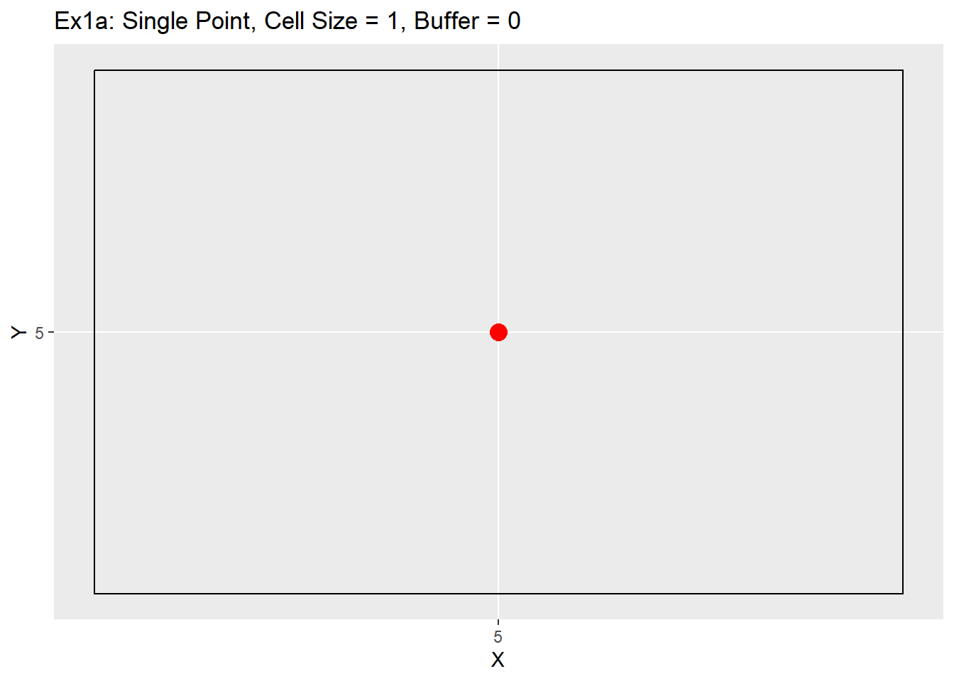
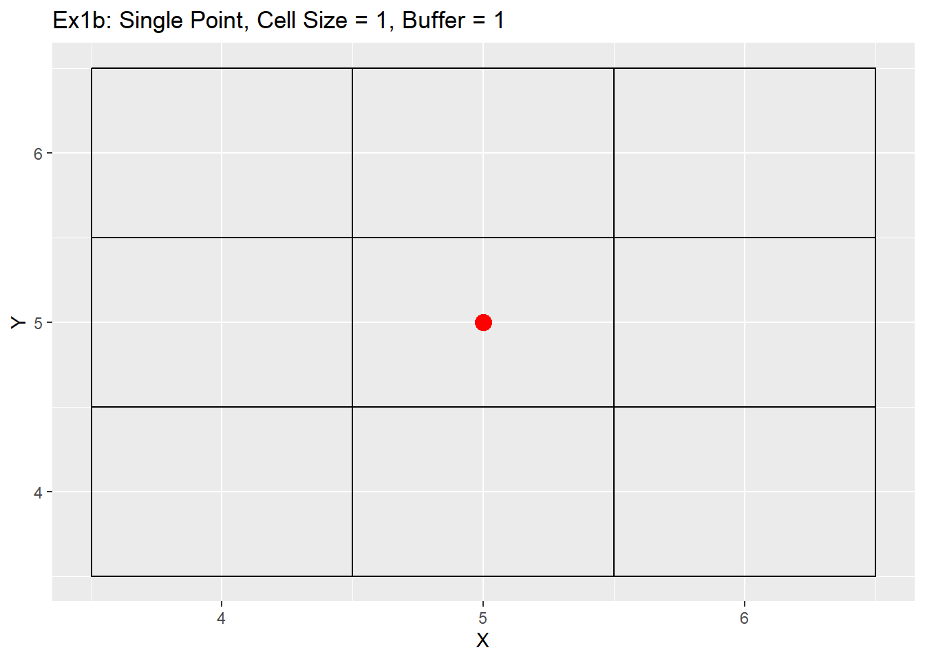
Below are a series of examples showing what the code can do, and also some items to be aware of when using the code. The first example will show a single point with and without a buffer. The point is located at 5,5, uses a 1 unit cell size, and a buffer of 0 and then of 1.
Ex1_Grid <- Make_Grid(x_coords = 5, y_coords = 5, cell_size = 1, buffer = 0)

ggplot() +
  geom_rect(data = Ex1_Grid, aes(xmin = x - cell_size/2, ymin = y - cell_size/2, xmax = x + cell_size/2, ymax = y + cell_size/2), color = 'black', fill = NA) +
  geom_point(data = data.table(X = 5, Y = 5), aes(x = X, y = Y), color = 'red', size = 4) +
  labs(title = 'Ex1a: Single Point, Cell Size = 1, Buffer = 0') +
  scale_x_continuous(breaks = seq(-20,20,1)) +
  scale_y_continuous(breaks = seq(-20,20,1))
Ex1_Grid <- Make_Grid(x_coords = 5, y_coords = 5, cell_size = 1, buffer = 1)

ggplot() +
  geom_rect(data = Ex1_Grid, aes(xmin = x - cell_size/2, ymin = y - cell_size/2, xmax = x + cell_size/2, ymax = y + cell_size/2), color = 'black', fill = NA) +
  geom_point(data = data.table(X = 5, Y = 5), aes(x = X, y = Y), color = 'red', size = 4) +
  labs(title = 'Ex1b: Single Point, Cell Size = 1, Buffer = 1') +
  scale_x_continuous(breaks = seq(-20,20,1)) +
  scale_y_continuous(breaks = seq(-20,20,1))
Next we will take a look at the actual output of the code.
Ex1_Grid
##    x y cell_size cell_id
## 1: 4 4         1       1
## 2: 4 5         1       2
## 3: 4 6         1       3
## 4: 5 4         1       4
## 5: 5 5         1       5
## 6: 5 6         1       6
## 7: 6 4         1       7
## 8: 6 5         1       8
## 9: 6 6         1       9
The output is a table with the cell node centers x and y coordinate, the size of the cell, and the cell id. As stated earlier, part of the goal was a simplistic output, that could easily be used in other applications. Using this output a spatial dataset could be made of the cell nodes, or as shown above turned into a grid in ggplot2. The main focus was to be able to locate each cell relative to on another and to know how big each cell is. The ids were added to make it easier to uniquely identify each cell if needed. That covers the basics of the first function and the general output of the code, which will stay the same throughout the process. Now we can move onto some more examples to show off first function.
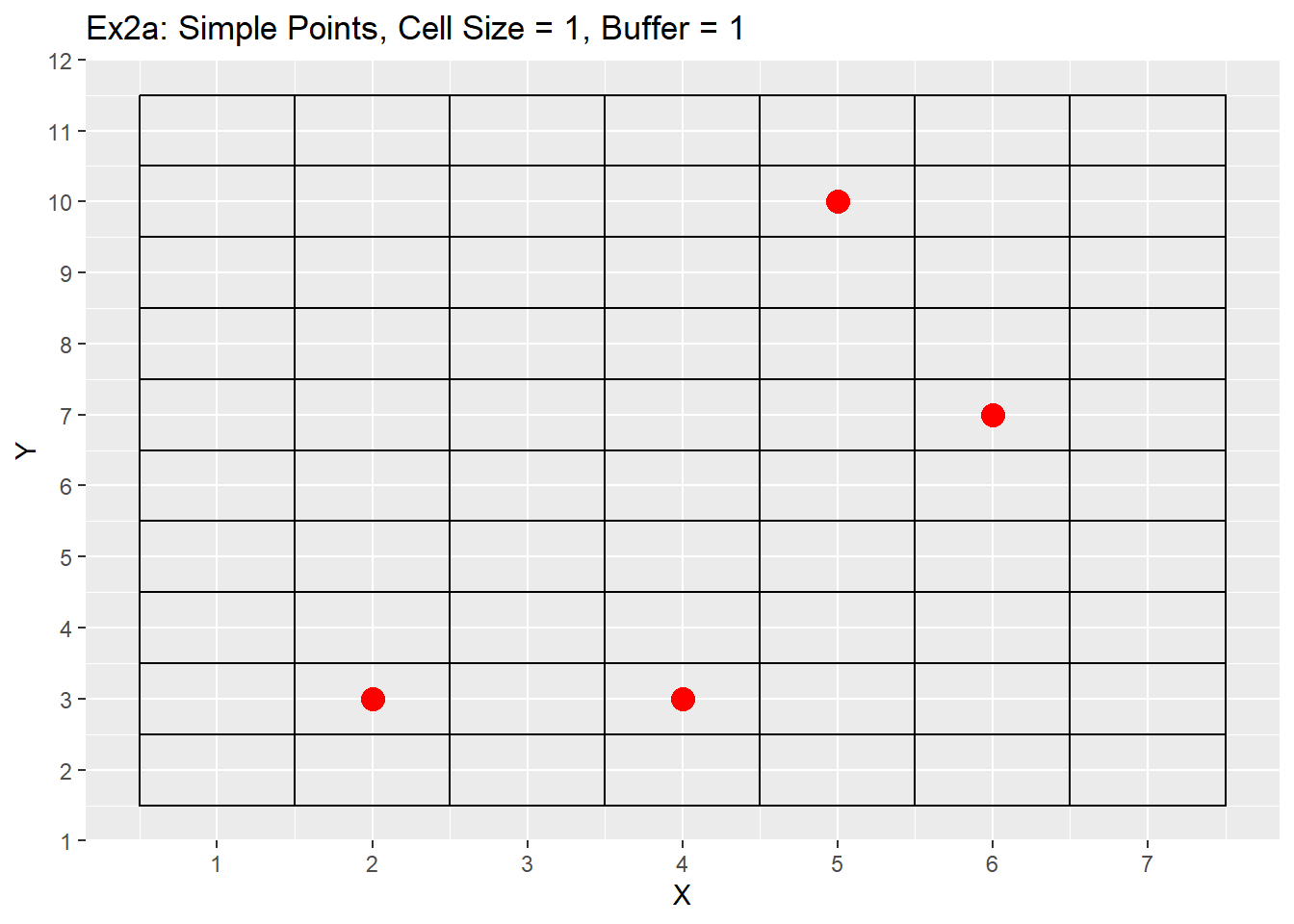
The second set of examples will use two different datasets, also located on my github page, that will be used throughout this post. The first is simply called simple_points, as it is just that. A series of 4 simple whole number points, meant to represent a very simplistic dataset, and the second called complex_points also contains 4 points but with a higher accuracy going into the decimal places. The second dataset is more representative of spatial or complex datasets in which we don’t expect to have nice round whole numbers.
# Reading in the datasets from my google drive
simple_points <- fread(input = 'https://drive.google.com/uc?export=download&id=1_QFxVmmu7Svkea_tlNa7lvlVYubiHZ2H')

simple_points
##    X  Y
## 1: 5 10
## 2: 4  3
## 3: 6  7
## 4: 2  3
Ex1_Grid <- Make_Grid(x_coords = simple_points$X, y_coords = simple_points$Y, cell_size = 1, buffer = 1)

ggplot() +
  geom_rect(data = Ex1_Grid, aes(xmin = x - cell_size/2, ymin = y - cell_size/2, xmax = x + cell_size/2, ymax = y + cell_size/2), color = 'black', fill = NA) +
  geom_point(data = simple_points, aes(x = X, y = Y), color = 'red', size = 4) +
  labs(title = 'Ex2a: Simple Points, Cell Size = 1, Buffer = 1') +
  scale_x_continuous(breaks = seq(-20,20,1)) +
  scale_y_continuous(breaks = seq(-20,20,1))
complex_points <- fread(input = 'https://drive.google.com/uc?export=download&id=16BUG50nHhOXoBRlDQYcYufvgTsG5_Df4')

complex_points
##           X        Y
## 1: 5.030643 9.364903
## 2: 3.947104 2.223640
## 3: 5.757131 6.623803
## 4: 1.208476 3.885082
Ex1_Grid <- Make_Grid(x_coords = complex_points$X, y_coords = complex_points$Y, cell_size = 1, buffer = 1)

ggplot() +
  geom_rect(data = Ex1_Grid, aes(xmin = x - cell_size/2, ymin = y - cell_size/2, xmax = x + cell_size/2, ymax = y + cell_size/2), color = 'black', fill = NA) +
  geom_point(data = complex_points, aes(x = X, y = Y), color = 'red', size = 4) +
  labs(title = 'Ex2b: Complex Points, Cell Size = 1, Buffer = 1') +
  scale_x_continuous(breaks = seq(-20,20,1)) +
  scale_y_continuous(breaks = seq(-20,20,1))
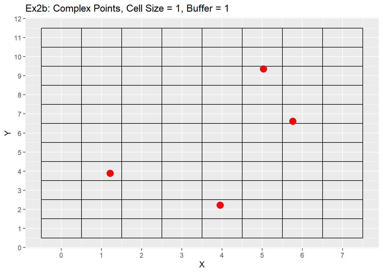
As you can see from the examples both produce fairly similar grids, but the simple dataset has all the points located in the center of each cell, while the complex points are all located within each cell. Both examples show the grids covering the entire extent of our area of interest and the additional buffer gives an additional rows and columns to each side of the grid. One last point is that while the cell size is 1 unit, the edges of each cell are located at 0.5 intervals. This is due to center the points within the cells. For example a cell located at 5,5 will have its edges located between 4.5 an 5.5, or 1 unit of length. This does appear strange, especially when we are use to origins located at zero, but as stated earlier my intentions were not so much making a nice grid as making a grid that fit the data provided. Next we will look at how changing both the number of buffers and cell size changes the grid. For these examples only the simple points data will be used.
Ex1_Grid <- Make_Grid(x_coords = simple_points$X, y_coords = simple_points$Y, cell_size = 1, buffer = 2)

ggplot() +
  geom_rect(data = Ex1_Grid, aes(xmin = x - cell_size/2, ymin = y - cell_size/2, xmax = x + cell_size/2, ymax = y + cell_size/2), color = 'black', fill = NA) +
  geom_point(data = complex_points, aes(x = X, y = Y), color = 'red', size = 4) +
  labs(title = 'Ex3a: Simple Points, Cell Size = 1, Buffer = 2') +
  scale_x_continuous(breaks = seq(-20,20,1)) +
  scale_y_continuous(breaks = seq(-20,20,1))
Ex1_Grid <- Make_Grid(x_coords = simple_points$X, y_coords = simple_points$Y, cell_size = 1, buffer = 4)

ggplot() +
  geom_rect(data = Ex1_Grid, aes(xmin = x - cell_size/2, ymin = y - cell_size/2, xmax = x + cell_size/2, ymax = y + cell_size/2), color = 'black', fill = NA) +
  geom_point(data = complex_points, aes(x = X, y = Y), color = 'red', size = 4) +
  labs(title = 'Ex3b: Simple Points, Cell Size = 1, Buffer = 4') +
  scale_x_continuous(breaks = seq(-20,20,1)) +
  scale_y_continuous(breaks = seq(-20,20,1))
Ex1_Grid <- Make_Grid(x_coords = simple_points$X, y_coords = simple_points$Y, cell_size = 4, buffer = 2)

ggplot() +
  geom_rect(data = Ex1_Grid, aes(xmin = x - cell_size/2, ymin = y - cell_size/2, xmax = x + cell_size/2, ymax = y + cell_size/2), color = 'black', fill = NA) +
  geom_point(data = complex_points, aes(x = X, y = Y), color = 'red', size = 4) +
  labs(title = 'Ex3c: Simple Points, Cell Size = 4, Buffer = 2') +
  scale_x_continuous(breaks = seq(-20,20,1)) +
  scale_y_continuous(breaks = seq(-20,20,1))
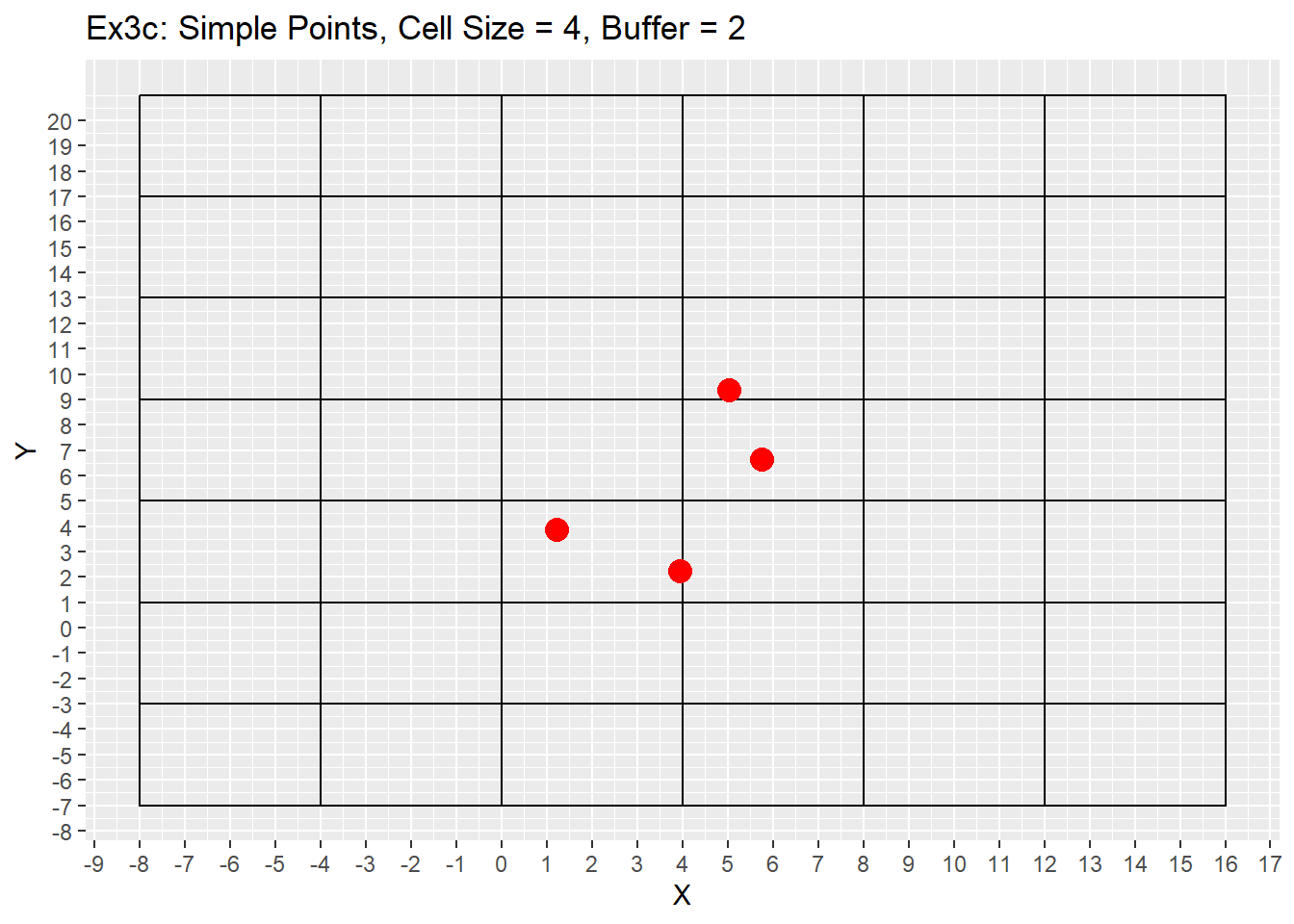
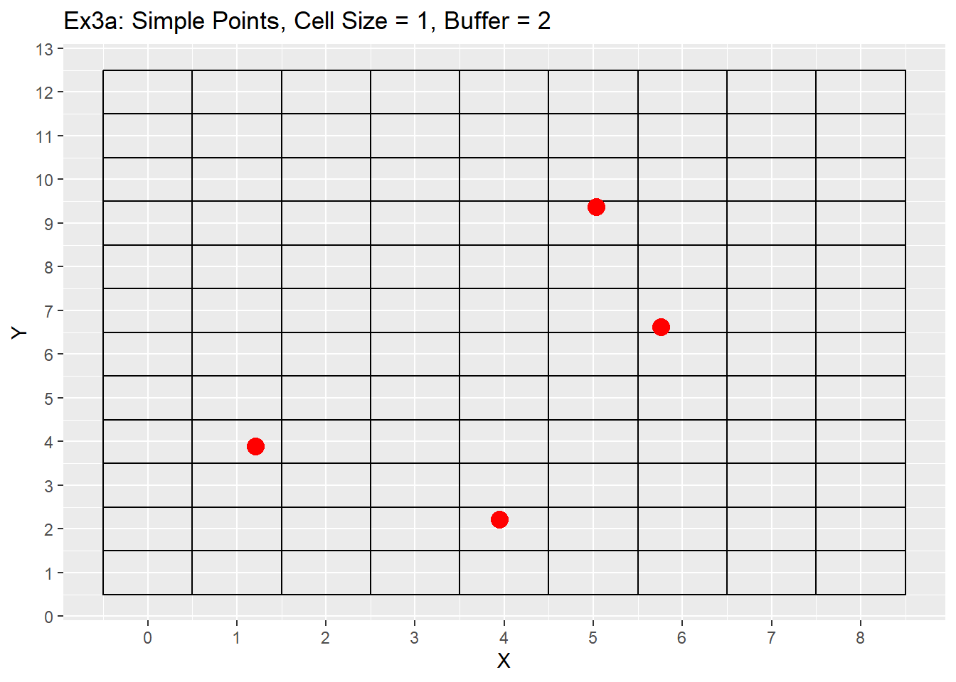
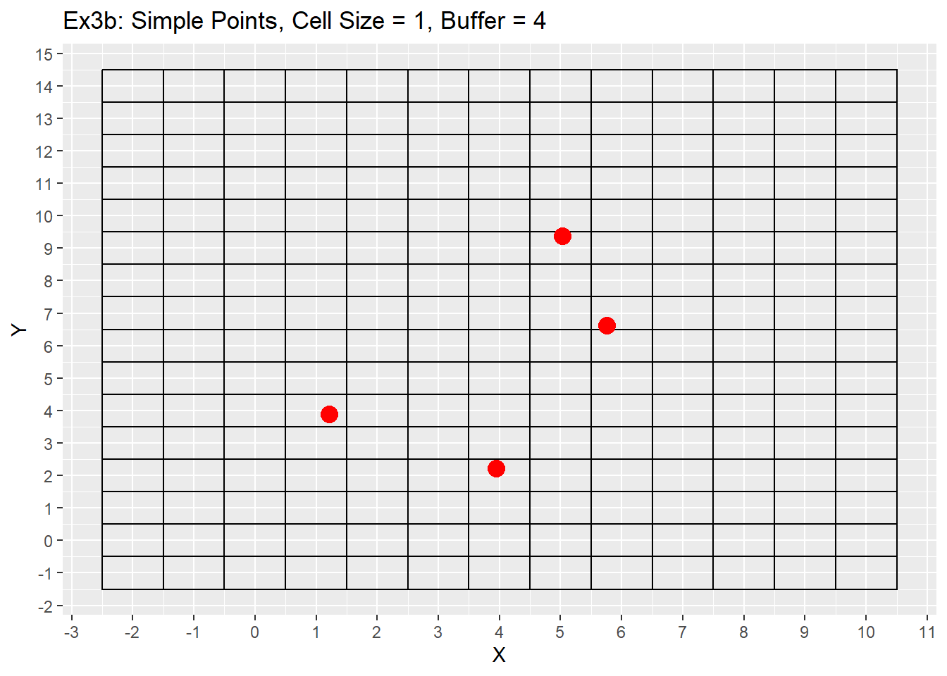
From the examples 3a to 3b the difference between the buffer size is apparent with the additional buffer providing a larger plotting area. Example 3c shows using a larger cell size of 4, which causes multiple points to be located in a single cell. This example will be revisited later showing off the grid refinement that will put each point within its own cell. The last consideration is the grid does not care about negative values and can make a grid with negative values if points are located in negative space, or the buffer value is large enough to go into negative space. As seen in example 3c as well.
Ghost Nodes
Ghost_Nodes_Alt <- function(Grid, x_coords, y_coords, ref_method){
  # method selection
  if (ref_method == 'Single') {
    Ghosts <- lapply(1:length(x_coords), function(a){
      temp_point_x <- x_coords[a]
      temp_point_y <- y_coords[a]
      temp_cell_size <- min(Grid$cell_size)
      # locate cell ids
      Grid_Nodes <- Grid[between(x = x, lower = temp_point_x-temp_cell_size/2, upper = temp_point_x+temp_cell_size/2, incbounds = T)][between(x = y, lower = temp_point_y-temp_cell_size/2, upper = temp_point_y+temp_cell_size/2, incbounds = T)]

      Grid_Nodes <- Grid_Nodes[cell_size == min(Grid_Nodes$cell_size)][1]

      Grid_Nodes
    })
    Ghosts_2 <- NA
  }else{

    if(ref_method != 'Radial'){return("No method found with that name. Please check spelling of the reference method")}
    # run for each point pair
    Ghosts <- lapply(1:length(x_coords), function(a){
      temp_point_x <- x_coords[a]
      temp_point_y <- y_coords[a]
      temp_cell_size <- min(Grid$cell_size)

      #find max/min x and y by multiplying the point location by 1.5 the current minimum distance in the grid
      min_x = temp_point_x - temp_cell_size*1.5
      min_y = temp_point_y - temp_cell_size*1.5
      max_x = temp_point_x + temp_cell_size*1.5
      max_y = temp_point_y + temp_cell_size*1.5

      # extract cell ids that will be needed
      Grid_Nodes <- Grid[between(x, min_x, max_x)][between(y, min_y, max_y)]
      Grid_Nodes
    })

    Ghosts_2 <- lapply(1:length(x_coords), function(a){
      temp_point_x <- x_coords[a]
      temp_point_y <- y_coords[a]
      temp_cell_size <- min(Grid$cell_size)

      #find max/min x and y by multiplying the point location by 1.5 the current minimum distance in the grid
      min_x = temp_point_x - temp_cell_size*1.5
      min_y = temp_point_y - temp_cell_size*1.5
      max_x = temp_point_x + temp_cell_size*1.5
      max_y = temp_point_y + temp_cell_size*1.5

      # extract cell ids that will be needed
      Grid_Nodes <- data.table('X' = c(min_x,max_x), 'Y' = c(min_y,max_y))
      Grid_Nodes
    })


  }
  Grid_Nodes <- rbindlist(Ghosts)
  Ghosts_2 <- rbindlist(Ghosts_2)
  list(Grid_Nodes, Ghosts_2)
}

Ghost_Nodes <- function(Grid, x_coords, y_coords, ref_method){
  # method selection
  if (ref_method == 'Single') {
    Ghosts <- lapply(1:length(x_coords), function(a){
      temp_point_x <- x_coords[a]
      temp_point_y <- y_coords[a]
      temp_cell_size <- min(Grid$cell_size)
      # locate cell ids
      Grid_Nodes <- Grid[between(x = x, lower = temp_point_x-temp_cell_size/2, upper = temp_point_x+temp_cell_size/2, incbounds = T)][between(x = y, lower = temp_point_y-temp_cell_size/2, upper = temp_point_y+temp_cell_size/2, incbounds = T)]

      Grid_Nodes <- Grid_Nodes[cell_size == min(Grid_Nodes$cell_size)][1]

      Grid_Nodes
    })
  }else{

    if(ref_method != 'Radial'){return("No method found with that name. Please check spelling of the reference method")}
    # run for each point pair
    Ghosts <- lapply(1:length(x_coords), function(a){
      temp_point_x <- x_coords[a]
      temp_point_y <- y_coords[a]
      temp_cell_size <- min(Grid$cell_size)

      #find max/min x and y by multiplying the point location by 1.5 the current minimum distance in the grid
      min_x = temp_point_x - temp_cell_size*1.5
      min_y = temp_point_y - temp_cell_size*1.5
      max_x = temp_point_x + temp_cell_size*1.5
      max_y = temp_point_y + temp_cell_size*1.5

      # extract cell ids that will be needed
      Grid_Nodes <- Grid[between(x, min_x, max_x)][between(y, min_y, max_y)]
      Grid_Nodes
    })
  }
  Grid_Nodes <- rbindlist(Ghosts)
  Grid_Nodes
}
The next section covers the ghost node code (seen above). I have put two different versions of the code in this post, but only provide the “Ghost_Nodes” code on Github. The alt version is just to provide additional output for plotting reasons in this post.
The ghost nodes code is used to find the extents around each point that need to be refined, and allows for two different methods in determining that extent. The first is called single cell refinement and simply returns the location the cell is located in as the cell to refine, and the second is called radial cell refinement. The second method finds the extent of 1.5 cells below and to the left, and 1.5 cells above to the right. All cells located within that area are returned as cells to be refined. This effectively selects all cells around the point. This generally amounts to 9 different cells chosen, but in the case when the point is located directly in the center that number increases to a total 16 cells with each refinement. Due to the special nature of being located in the very center of the cell, the code does not make an assumption of which cell to use to represent the point, but instead takes all cells around it. My assumption is that this will be a rare case and should not occur often, and if it does the code will still refine the cells around the point. The user will then need to decide which cell around the point is the best to represent the point location. The code output for both methods is a table of the cell ids of the cells to be refined, which is used as an input for the next function.
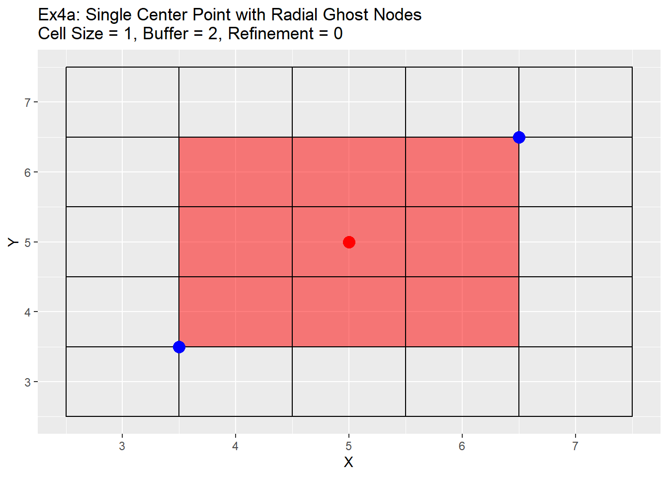
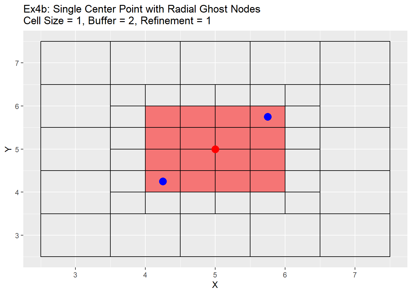
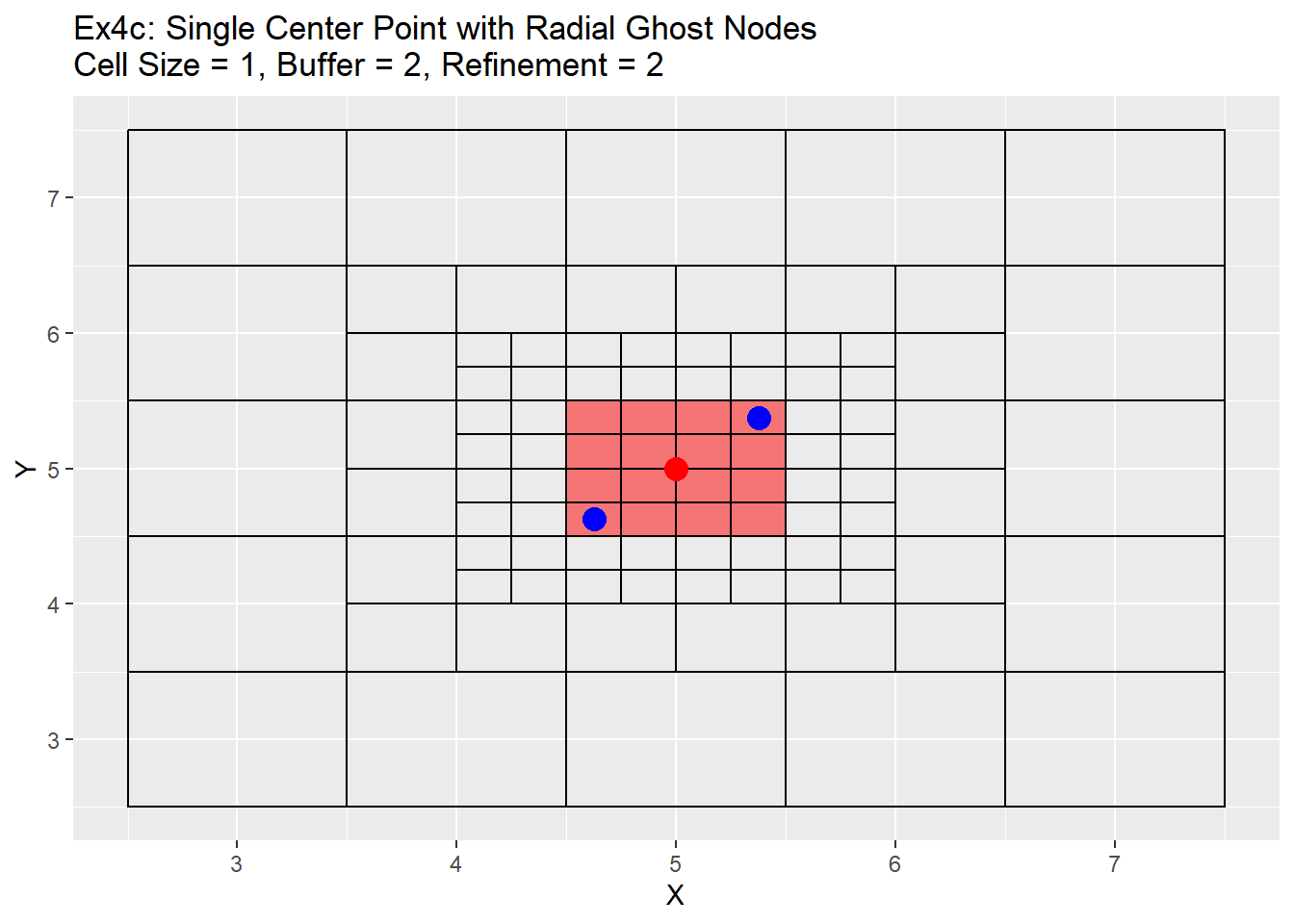
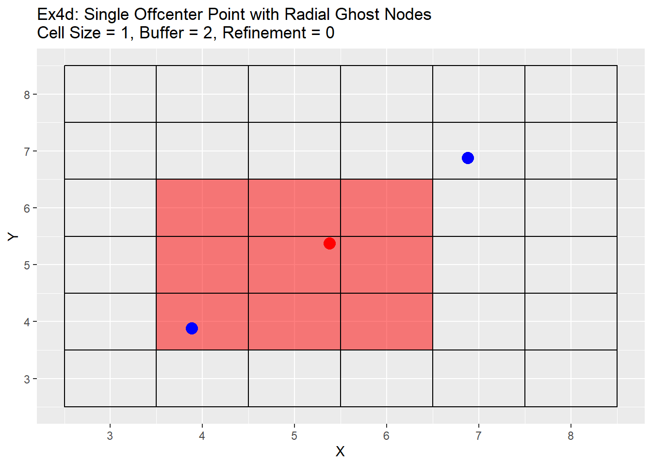
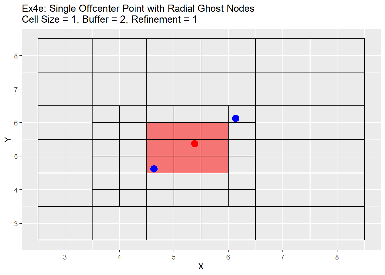
Because the single refinement is an easy concept to understand, only the radial method examples will be shown below. Two series of examples are shown below. The first is showing the case in which the point is located directly in the center at location 5,5 and the second shows a more realistic point located at 5.38,5.38. In both cases a two level refinement will occur to show off the process. For each graph the the point we want to refine is shown in red, the blue points are the corners of the area we wish to refine, and the read filled cells is the area between the blue points that will be refined.
Ex2_Grid <- Make_Grid(x_coords = 5, y_coords = 5, cell_size = 1, buffer = 2)

Ex2_Ghosts <- Ghost_Nodes_Alt(Grid = Ex2_Grid, x_coords = 5, y_coords = 5, ref_method = 'Radial')

ggplot() +
  geom_rect(data = Ex2_Grid, aes(xmin = x - cell_size/2, ymin = y - cell_size/2, xmax = x + cell_size/2, ymax = y + cell_size/2), color = 'black', fill = NA) +
  geom_rect(data = Ex2_Ghosts[[1]], aes(xmin = x - cell_size/2, ymin = y - cell_size/2, xmax = x + cell_size/2, ymax = y + cell_size/2), color = 'black', fill = 'red', alpha = 0.5) +
  geom_point(data = data.table(X = 5, Y = 5), aes(x = X, y = Y), color = 'red', size = 4) +
  geom_point(data = Ex2_Ghosts[[2]], aes(x = X, y = Y), color = 'blue', size = 4) +
  labs(title = 'Ex4a: Single Center Point with Radial Ghost Nodes\nCell Size = 1, Buffer = 2, Refinement = 0') +
  scale_x_continuous(breaks = seq(-20,20,1)) +
  scale_y_continuous(breaks = seq(-20,20,1))
Ex2_Quad_Tree <- Quad_Tree(Grid = Ex2_Grid, ghost_nodes = Ex2_Ghosts[[1]])

Ex2_Ghosts <- Ghost_Nodes_Alt(Grid = Ex2_Quad_Tree, x_coords = 5, y_coords = 5, ref_method = 'Radial')

ggplot() +
  geom_rect(data = Ex2_Quad_Tree, aes(xmin = x - cell_size/2, ymin = y - cell_size/2, xmax = x + cell_size/2, ymax = y + cell_size/2), color = 'black', fill = NA) +
  geom_rect(data = Ex2_Ghosts[[1]], aes(xmin = x - cell_size/2, ymin = y - cell_size/2, xmax = x + cell_size/2, ymax = y + cell_size/2), color = 'black', fill = 'red', alpha = 0.5) +
  geom_point(data = data.table(X = 5, Y = 5), aes(x = X, y = Y), color = 'red', size = 4) +
  geom_point(data = Ex2_Ghosts[[2]], aes(x = X, y = Y), color = 'blue', size = 4) +
  labs(title = 'Ex4b: Single Center Point with Radial Ghost Nodes\nCell Size = 1, Buffer = 2, Refinement = 1') +
  scale_x_continuous(breaks = seq(-20,20,1)) +
  scale_y_continuous(breaks = seq(-20,20,1))
Ex2_Quad_Tree <- Quad_Tree(Grid = Ex2_Quad_Tree, ghost_nodes = Ex2_Ghosts[[1]])

Ex2_Ghosts <- Ghost_Nodes_Alt(Grid = Ex2_Quad_Tree, x_coords = 5, y_coords = 5, ref_method = 'Radial')

ggplot() +
  geom_rect(data = Ex2_Quad_Tree, aes(xmin = x - cell_size/2, ymin = y - cell_size/2, xmax = x + cell_size/2, ymax = y + cell_size/2), color = 'black', fill = NA) +
  geom_rect(data = Ex2_Ghosts[[1]], aes(xmin = x - cell_size/2, ymin = y - cell_size/2, xmax = x + cell_size/2, ymax = y + cell_size/2), color = 'black', fill = 'red', alpha = 0.5) +
  geom_point(data = data.table(X = 5, Y = 5), aes(x = X, y = Y), color = 'red', size = 4) +
  geom_point(data = Ex2_Ghosts[[2]], aes(x = X, y = Y), color = 'blue', size = 4) +
  labs(title = 'Ex4c: Single Center Point with Radial Ghost Nodes\nCell Size = 1, Buffer = 2, Refinement = 2') +
  scale_x_continuous(breaks = seq(-20,20,1)) +
  scale_y_continuous(breaks = seq(-20,20,1))
##################

Ex2_Grid <- Make_Grid(x_coords = 5.38, y_coords = 5.38, cell_size = 1, buffer = 2)

Ex2_Ghosts <- Ghost_Nodes_Alt(Grid = Ex2_Grid, x_coords = 5.38, y_coords = 5.38, ref_method = 'Radial')

ggplot() +
  geom_rect(data = Ex2_Grid, aes(xmin = x - cell_size/2, ymin = y - cell_size/2, xmax = x + cell_size/2, ymax = y + cell_size/2), color = 'black', fill = NA) +
  geom_rect(data = Ex2_Ghosts[[1]], aes(xmin = x - cell_size/2, ymin = y - cell_size/2, xmax = x + cell_size/2, ymax = y + cell_size/2), color = 'black', fill = 'red', alpha = 0.5) +
  geom_point(data = data.table(X = 5.38, Y = 5.38), aes(x = X, y = Y), color = 'red', size = 4) +
  geom_point(data = Ex2_Ghosts[[2]], aes(x = X, y = Y), color = 'blue', size = 4) +
  labs(title = 'Ex4d: Single Offcenter Point with Radial Ghost Nodes\nCell Size = 1, Buffer = 2, Refinement = 0') +
  scale_x_continuous(breaks = seq(-20,20,1)) +
  scale_y_continuous(breaks = seq(-20,20,1))
Ex2_Quad_Tree <- Quad_Tree(Grid = Ex2_Grid, ghost_nodes = Ex2_Ghosts[[1]])

Ex2_Ghosts <- Ghost_Nodes_Alt(Grid = Ex2_Quad_Tree, x_coords = 5.38, y_coords = 5.38, ref_method = 'Radial')

ggplot() +
  geom_rect(data = Ex2_Quad_Tree, aes(xmin = x - cell_size/2, ymin = y - cell_size/2, xmax = x + cell_size/2, ymax = y + cell_size/2), color = 'black', fill = NA) +
  geom_rect(data = Ex2_Ghosts[[1]], aes(xmin = x - cell_size/2, ymin = y - cell_size/2, xmax = x + cell_size/2, ymax = y + cell_size/2), color = 'black', fill = 'red', alpha = 0.5) +
  geom_point(data = data.table(X = 5.38, Y = 5.38), aes(x = X, y = Y), color = 'red', size = 4) +
  geom_point(data = Ex2_Ghosts[[2]], aes(x = X, y = Y), color = 'blue', size = 4) +
  labs(title = 'Ex4e: Single Offcenter Point with Radial Ghost Nodes\nCell Size = 1, Buffer = 2, Refinement = 1') +
  scale_x_continuous(breaks = seq(-20,20,1)) +
  scale_y_continuous(breaks = seq(-20,20,1))
Ex2_Quad_Tree <- Quad_Tree(Grid = Ex2_Quad_Tree, ghost_nodes = Ex2_Ghosts[[1]])

Ex2_Ghosts <- Ghost_Nodes_Alt(Grid = Ex2_Quad_Tree, x_coords = 5.38, y_coords = 5.38, ref_method = 'Radial')

ggplot() +
  geom_rect(data = Ex2_Quad_Tree, aes(xmin = x - cell_size/2, ymin = y - cell_size/2, xmax = x + cell_size/2, ymax = y + cell_size/2), color = 'black', fill = NA) +
  geom_rect(data = Ex2_Ghosts[[1]], aes(xmin = x - cell_size/2, ymin = y - cell_size/2, xmax = x + cell_size/2, ymax = y + cell_size/2), color = 'black', fill = 'red', alpha = 0.5) +
  geom_point(data = data.table(X = 5.38, Y = 5.38), aes(x = X, y = Y), color = 'red', size = 4) +
  geom_point(data = Ex2_Ghosts[[2]], aes(x = X, y = Y), color = 'blue', size = 4) +
  labs(title = 'Ex4f: Single Offcenter Point with Radial Ghost Nodes\nCell Size = 1, Buffer = 2, Refinement = 2') +
  scale_x_continuous(breaks = seq(-20,20,1)) +
  scale_y_continuous(breaks = seq(-20,20,1))
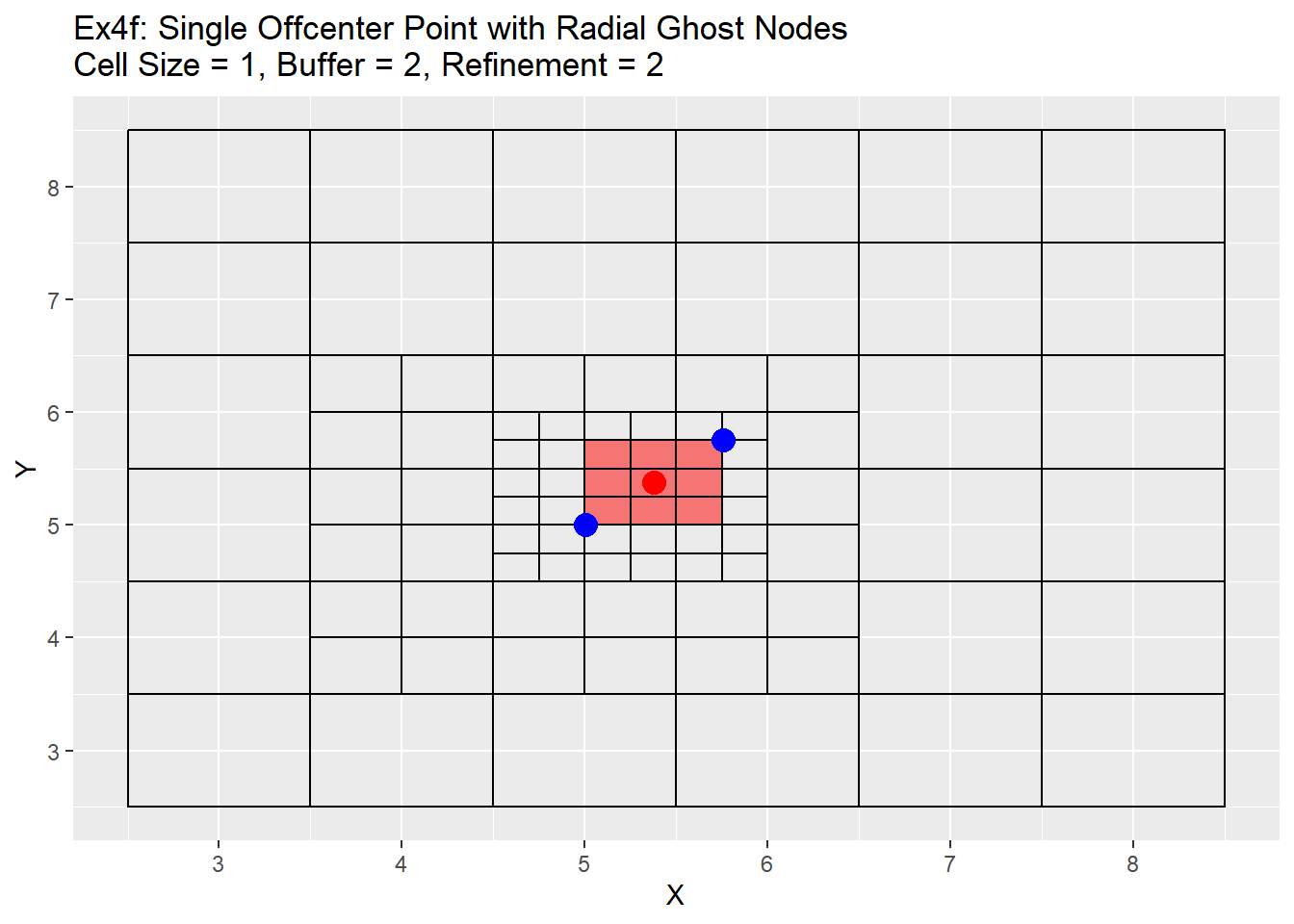
The graphs show the change in the refinement of the cells. Starting with the single center graphs, graph 4a shows the code is working as intended with 9 cells chosen for refinement. As we go to graph 4b we see that the cells selected in the previous graph have all been refined, and a new set of cells from the refined cells is now chosen. The number of cells chosen is now 16. The reason for this is that the blue points are also located exactly in the center of the cells, and when trying to choose weather to include the cell or not for refinement cannot be determined and errs on the side of caution and includes the cell. This is repeated in graph 4c, in which another 16 cells are chosen for refinement. Once again I believe this should be a fairly rare case in which a point lines up exactly with the grid center, but wanted to show it for clarification and in case a situation like this does occur. Graph 4d shows the off-center point and like graph 4a selects only 9 cells, but this time you can see how the blue points are also located off-center. The blue point on the bottom left side is our lower and left side boundary. Any cell centers that are above and to the right of that point will be selected. The top right blue point is our top and right boundary. Any cell centers below and to the left will be selected. The cells that cross over between those to selection process are the cells that will be refined (shown in red). Graph 4e shows first refinement step, and in this case only 9 cells are selected for further refinement. This is the intended output and should be the normal case for most situations. The last graph 4f shows the second refinement and once again only 9 cells for further refinement selected. During this process the change in cell size will not be uniform like when the point is located directly in the middle of the cell. As in the graph 4e has two cells on the left hand side of the grid that are of a 0.5 cell size, and only one on the right hand side.
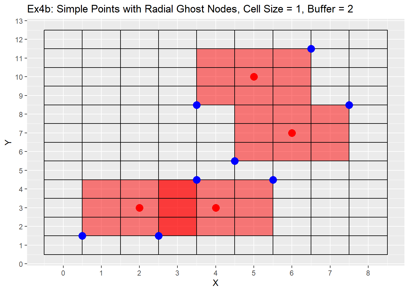
The second set of examples for ghost nodes code shows the case using the simple points dataset. In this case we will have overlapping cells, but the code will not have any issues with that as all the cells to be refined are removed at once and then refined and not refined by point. Therefore no cell is accidentally refined twice. The output is the same table as the output for for the make grid function, with just the cells to be refined. For clarification the normal output is just a table and not a list, the list is used here with the alt code in order to plot the blue points.
Ex2_Grid <- Make_Grid(x_coords = simple_points$X, y_coords = simple_points$Y, cell_size = 1, buffer = 2)

Ex2_Ghosts <- Ghost_Nodes_Alt(Grid = Ex2_Grid, x_coords = simple_points$X, y_coords = simple_points$Y, ref_method = 'Radial')

Ex2_Ghosts[[1]]
##     x  y cell_size cell_id
##  1: 4  9         1      57
##  2: 4 10         1      58
##  3: 4 11         1      59
##  4: 5  9         1      69
##  5: 5 10         1      70
##  6: 5 11         1      71
##  7: 6  9         1      81
##  8: 6 10         1      82
##  9: 6 11         1      83
## 10: 3  2         1      38
## 11: 3  3         1      39
## 12: 3  4         1      40
## 13: 4  2         1      50
## 14: 4  3         1      51
## 15: 4  4         1      52
## 16: 5  2         1      62
## 17: 5  3         1      63
## 18: 5  4         1      64
## 19: 5  6         1      66
## 20: 5  7         1      67
## 21: 5  8         1      68
## 22: 6  6         1      78
## 23: 6  7         1      79
## 24: 6  8         1      80
## 25: 7  6         1      90
## 26: 7  7         1      91
## 27: 7  8         1      92
## 28: 1  2         1      14
## 29: 1  3         1      15
## 30: 1  4         1      16
## 31: 2  2         1      26
## 32: 2  3         1      27
## 33: 2  4         1      28
## 34: 3  2         1      38
## 35: 3  3         1      39
## 36: 3  4         1      40
##     x  y cell_size cell_id
ggplot() +
  geom_rect(data = Ex2_Grid, aes(xmin = x - cell_size/2, ymin = y - cell_size/2, xmax = x + cell_size/2, ymax = y + cell_size/2), color = 'black', fill = NA) +
  geom_rect(data = Ex2_Ghosts[[1]], aes(xmin = x - cell_size/2, ymin = y - cell_size/2, xmax = x + cell_size/2, ymax = y + cell_size/2), color = 'black', fill = 'red', alpha = 0.5) +
  geom_point(data = data.table(X = simple_points$X, Y = simple_points$Y), aes(x = X, y = Y), color = 'red', size = 4) +
  geom_point(data = Ex2_Ghosts[[2]], aes(x = X, y = Y), color = 'blue', size = 4) +
  labs(title = 'Ex4b: Simple Points with Radial Ghost Nodes, Cell Size = 1, Buffer = 2') +
  scale_x_continuous(breaks = seq(-20,20,1)) +
  scale_y_continuous(breaks = seq(-20,20,1))
Quad Tree
Quad_Tree <- function(Grid, ghost_nodes){
    # this is the outer loop that controls the number of refinements to do
    # using ghost nodes refine grid down number of steps desired
    new_cells <- lapply(ghost_nodes$cell_id, function(b) {
        temp_grid <- Grid[cell_id == b]
        # reduce each side by 2
        new_cell1 = data.table(x = temp_grid$x + temp_grid$cell_size/4, y = temp_grid$y + temp_grid$cell_size/4, cell_size = temp_grid$cell_size/2, cell_id = 0)
        new_cell2 = data.table(x = temp_grid$x + temp_grid$cell_size/4, y = temp_grid$y - temp_grid$cell_size/4, cell_size = temp_grid$cell_size/2, cell_id = 0)
        new_cell3 = data.table(x = temp_grid$x - temp_grid$cell_size/4, y = temp_grid$y - temp_grid$cell_size/4, cell_size = temp_grid$cell_size/2, cell_id = 0)
        new_cell4 = data.table(x = temp_grid$x - temp_grid$cell_size/4, y = temp_grid$y + temp_grid$cell_size/4, cell_size = temp_grid$cell_size/2, cell_id = 0)
        new_cells <- rbindlist(list(new_cell1,new_cell2, new_cell3, new_cell4))
    })
    # remove old cells and add in new cells, order by x and then y
    new_cells <- rbindlist(new_cells)
    Grid <- Grid[!cell_id %in% ghost_nodes$cell_id]
    Grid <- rbind(Grid, new_cells)
    Grid <- Grid[order(x,y)]
    Grid$cell_id <- 1:nrow(Grid)
    Grid
}
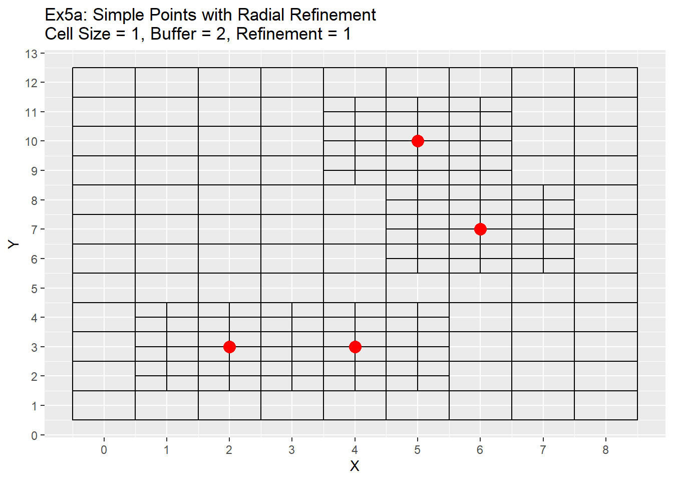
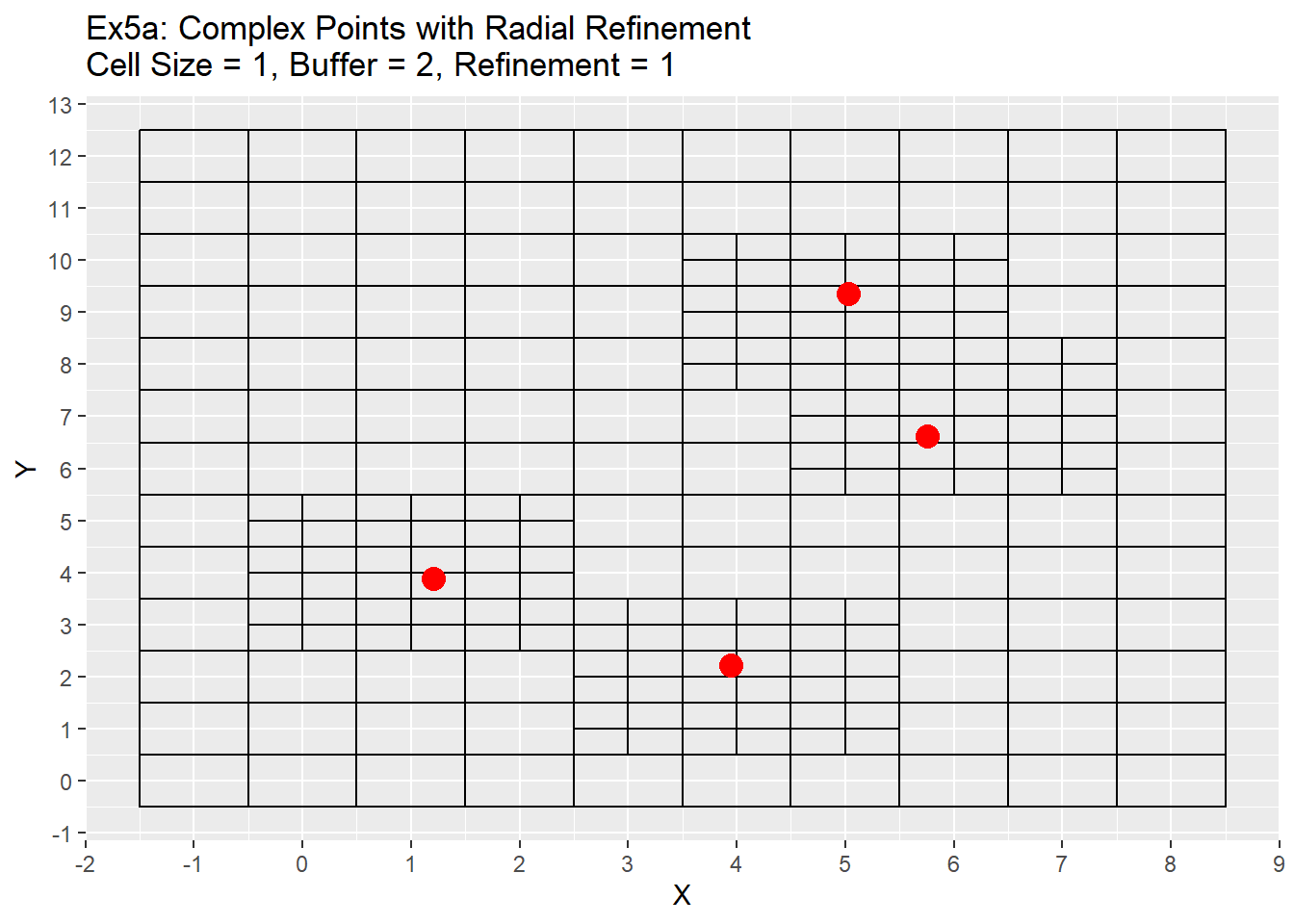
The quad tree function (above) takes the grid table and the ghost node table as inputs, and then refines the cells at the ghost node locations. The code loops through all ghost nodes and turns the cell locations at those nodes into 4 equal parts. It does this by taking the ghost node centroid value and adding or subtracting the quarter distance of the current cell size to create four new centroids. The cell size is then set to half the cell size and the cell id is set to zero as a placeholder. The new refined grids are then inserted into the original grid table, the ghost nodes are removed, and new ids are created for the new grid. The output is the same, a table of the centroids, cell size, and cell id.
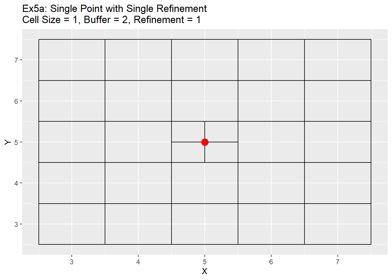
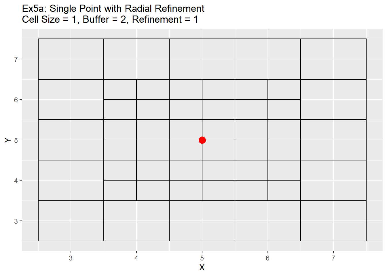
Below are a series of examples showing a single point example (5,5), simple points, complex points, and both the single and radial refinement methods.
Ex3_Grid <- Make_Grid(x_coords = 5, y_coords = 5, cell_size = 1, buffer = 2)

Ex3_Ghosts <- Ghost_Nodes(Grid = Ex3_Grid, x_coords = 5, y_coords = 5, ref_method = 'Single')

Ex3_Quad_Tree <- Quad_Tree(Grid = Ex3_Grid, ghost_nodes = Ex3_Ghosts)

ggplot() +
  geom_rect(data = Ex3_Quad_Tree, aes(xmin = x - cell_size/2, ymin = y - cell_size/2, xmax = x + cell_size/2, ymax = y + cell_size/2), color = 'black', fill = NA) +
  geom_point(data = data.table(X = 5, Y = 5), aes(x = X, y = Y), color = 'red', size = 4) +
  labs(title = 'Ex5a: Single Point with Single Refinement\nCell Size = 1, Buffer = 2, Refinement = 1') +
  scale_x_continuous(breaks = seq(-20,20,1)) +
  scale_y_continuous(breaks = seq(-20,20,1))
# Radial single point
Ex3_Grid <- Make_Grid(x_coords = 5, y_coords = 5, cell_size = 1, buffer = 2)

Ex3_Ghosts <- Ghost_Nodes(Grid = Ex3_Grid, x_coords = 5, y_coords = 5, ref_method = 'Radial')

Ex3_Quad_Tree <- Quad_Tree(Grid = Ex3_Grid, ghost_nodes = Ex3_Ghosts)

ggplot() +
  geom_rect(data = Ex3_Quad_Tree, aes(xmin = x - cell_size/2, ymin = y - cell_size/2, xmax = x + cell_size/2, ymax = y + cell_size/2), color = 'black', fill = NA) +
  geom_point(data = data.table(X = 5, Y = 5), aes(x = X, y = Y), color = 'red', size = 4) +
  labs(title = 'Ex5a: Single Point with Radial Refinement\nCell Size = 1, Buffer = 2, Refinement = 1') +
  scale_x_continuous(breaks = seq(-20,20,1)) +
  scale_y_continuous(breaks = seq(-20,20,1))
# Simple Points, Radial
Ex3_Grid <- Make_Grid(x_coords = simple_points$X, y_coords = simple_points$Y, cell_size = 1, buffer = 2)

Ex3_Ghosts <- Ghost_Nodes(Grid = Ex3_Grid, x_coords = simple_points$X, y_coords = simple_points$Y, ref_method = 'Radial')

Ex3_Quad_Tree <- Quad_Tree(Grid = Ex3_Grid, ghost_nodes = Ex3_Ghosts)

ggplot() +
  geom_rect(data = Ex3_Quad_Tree, aes(xmin = x - cell_size/2, ymin = y - cell_size/2, xmax = x + cell_size/2, ymax = y + cell_size/2), color = 'black', fill = NA) +
  geom_point(data = data.table(X = simple_points$X, Y = simple_points$Y), aes(x = X, y = Y), color = 'red', size = 4) +
  labs(title = 'Ex5a: Simple Points with Radial Refinement\nCell Size = 1, Buffer = 2, Refinement = 1') +
  scale_x_continuous(breaks = seq(-20,20,1)) +
  scale_y_continuous(breaks = seq(-20,20,1))
# Complex Points, Radial
Ex3_Grid <- Make_Grid(x_coords = complex_points$X, y_coords = complex_points$Y, cell_size = 1, buffer = 2)

Ex3_Ghosts <- Ghost_Nodes(Grid = Ex3_Grid, x_coords = complex_points$X, y_coords = complex_points$Y, ref_method = 'Radial')

Ex3_Quad_Tree <- Quad_Tree(Grid = Ex3_Grid, ghost_nodes = Ex3_Ghosts)

ggplot() +
  geom_rect(data = Ex3_Quad_Tree, aes(xmin = x - cell_size/2, ymin = y - cell_size/2, xmax = x + cell_size/2, ymax = y + cell_size/2), color = 'black', fill = NA) +
  geom_point(data = data.table(X = complex_points$X, Y = complex_points$Y), aes(x = X, y = Y), color = 'red', size = 4) +
  labs(title = 'Ex5a: Complex Points with Radial Refinement\nCell Size = 1, Buffer = 2, Refinement = 1') +
  scale_x_continuous(breaks = seq(-20,20,1)) +
  scale_y_continuous(breaks = seq(-20,20,1))
Grid Refinement Main Function
Grid_Refinement_Function <- function(x_coords, y_coords, cell_size, buffer, num_ref, ref_method) {
    temp_grid <- Make_Grid(x_coords = x_coords, y_coords = y_coords, cell_size = cell_size, buffer = buffer)
    # check if refinement number is zero and return normal grid
    if (num_ref > 0){
        # now we enter into the refine grid loop
        for (i in 1:num_ref){
            # first find the ghost nodes
            ghosts <- Ghost_Nodes(Grid = temp_grid, x_coords = x_coords, y_coords = y_coords, ref_method = ref_method)
            # then run quad tree refinement
            temp_grid <- Quad_Tree(Grid = temp_grid, ghost_nodes = ghosts)
        }
    }
    # if no more refinements return the updated grid
    temp_grid
}
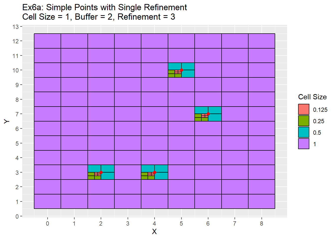
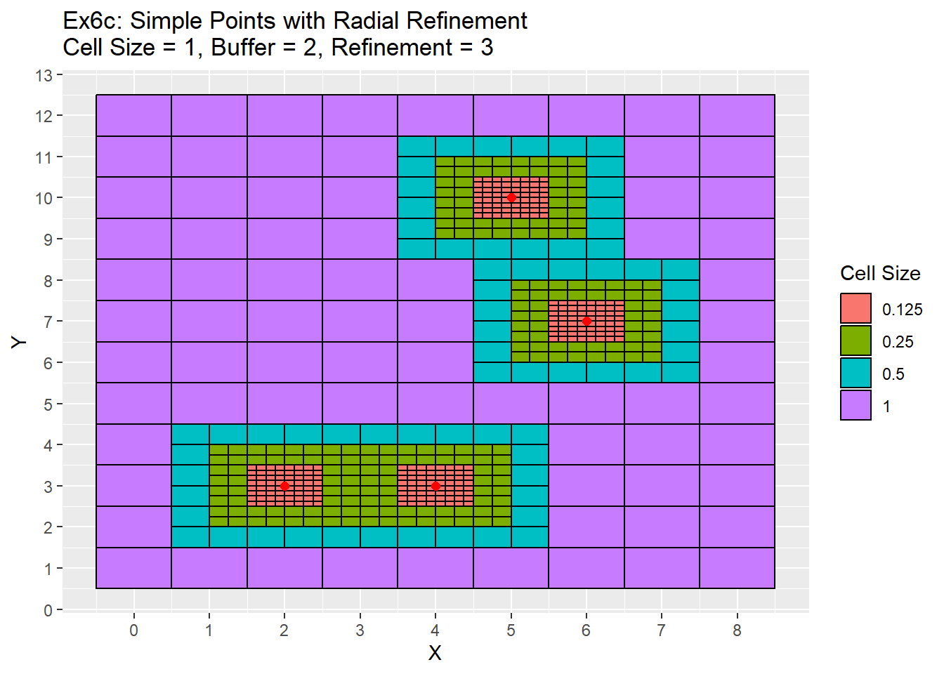
This is the main function that combines all previous functions into one simple to use function. It requires the x and y coordinates of the points, the desired cell size, number of buffers around the grid, the number of refinements to make, and the refinement method. Below are two examples, the first shows the simple points using a single refinement method and the second shows the radial refinement method. The cell sizes have been colored by size to highlight the refinement process.
# Ex5 Refinement Function Example
Ex5_Grid <- Grid_Refinement_Function(x_coords = simple_points$X, y_coords = simple_points$Y, cell_size = 1, buffer = 2, num_ref = 3, ref_method = 'Single')

ggplot() +
  geom_rect(data = Ex5_Grid, aes(xmin = x - cell_size/2, ymin = y - cell_size/2, xmax = x + cell_size/2, ymax = y + cell_size/2, fill = as.character(cell_size)), color = 'black') +
  geom_point(data = simple_points, aes(x = X, y = Y), color = 'red', size = 2) +
  labs(title = 'Ex6a: Simple Points with Single Refinement\nCell Size = 1, Buffer = 2, Refinement = 3', fill = 'Cell Size') +
  scale_x_continuous(breaks = seq(-20,20,1)) +
  scale_y_continuous(breaks = seq(-20,20,1))
Ex6_Grid <- Grid_Refinement_Function(x_coords = complex_points$X, y_coords = complex_points$Y, cell_size = 1, buffer = 2, num_ref = 3, ref_method = 'Single')

ggplot() +
  geom_rect(data = Ex6_Grid, aes(xmin = x - cell_size/2, ymin = y - cell_size/2, xmax = x + cell_size/2, ymax = y + cell_size/2, fill = as.character(cell_size)), color = 'black') +
  geom_point(data = complex_points, aes(x = X, y = Y), color = 'red', size = 2) +
  labs(title = 'Ex6b: Complex Points with Single Refinement\nCell Size = 1, Buffer = 2, Refinement = 3', fill = 'Cell Size') +
  scale_x_continuous(breaks = seq(-20,20,1)) +
  scale_y_continuous(breaks = seq(-20,20,1))
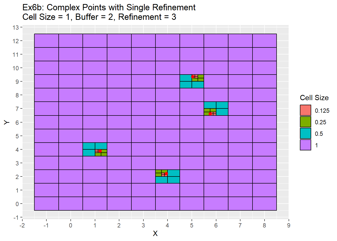
One item to note is that in the example 6a all refinements occurred in the bottom left quadrant. This is due to the simple points being located exactly in the center of each cell. Therefore a quadrant needs to be chosen during the ghost nodes function call in order for the refinement to proceed. This is the issue mentioned earlier in the grid function section. I have chosen the lower left quadrant to refine, but there is no technical reason any other quadrant could not be used as well. When you don’t have points located directly in the cell as in the case of the complex points in example 6b, then this is no longer an issue. The next two examples shows the same two examples above, but use the radial refinement method.
#Ex 6
Ex5_Grid <- Grid_Refinement_Function(x_coords = simple_points$X, y_coords = simple_points$Y, cell_size = 1, buffer = 2, num_ref = 3, ref_method = 'Radial')

ggplot() +
  geom_rect(data = Ex5_Grid, aes(xmin = x - cell_size/2, ymin = y - cell_size/2, xmax = x + cell_size/2, ymax = y + cell_size/2, fill = as.character(cell_size)), color = 'black') +
  geom_point(data = simple_points, aes(x = X, y = Y), color = 'red', size = 2) +
  labs(title = 'Ex6c: Simple Points with Radial Refinement\nCell Size = 1, Buffer = 2, Refinement = 3', fill = 'Cell Size') +
  scale_x_continuous(breaks = seq(-20,20,1)) +
  scale_y_continuous(breaks = seq(-20,20,1))
Ex6_Grid <- Grid_Refinement_Function(x_coords = complex_points$X, y_coords = complex_points$Y, cell_size = 1, buffer = 2, num_ref = 3, ref_method = 'Radial')

ggplot() +
  geom_rect(data = Ex6_Grid, aes(xmin = x - cell_size/2, ymin = y - cell_size/2, xmax = x + cell_size/2, ymax = y + cell_size/2, fill = as.character(cell_size)), color = 'black') +
  geom_point(data = complex_points, aes(x = X, y = Y), color = 'red', size = 2) +
  labs(title = 'Ex6d: Complex Points with Radial Refinement\nCell Size = 1, Buffer = 2, Refinement = 3', fill = 'Cell Size') +
  scale_x_continuous(breaks = seq(-20,20,1)) +
  scale_y_continuous(breaks = seq(-20,20,1))
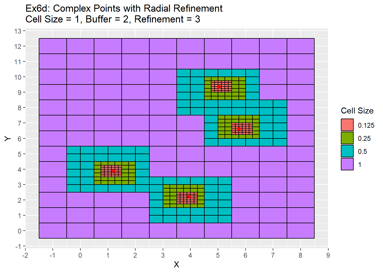
Once again the difference is between the two examples is that the simple points are located in the center of the cells. Therefore the refinement process is also centered which creates centered refinement zones. In the complex example, the refinements all appear bit off as they are not completely centered.
The next example is to show what a final output would look like when using main function.
Ex6_Grid <- Grid_Refinement_Function(x_coords = complex_points$X, y_coords = complex_points$Y, cell_size = 1, buffer = 2, num_ref = 3, ref_method = 'Radial')

Ex6_Grid
##       x  y cell_size cell_id
##   1: -1  0         1       1
##   2: -1  1         1       2
##   3: -1  2         1       3
##   4: -1  3         1       4
##   5: -1  4         1       5
##  ---
## 452:  8  8         1     452
## 453:  8  9         1     453
## 454:  8 10         1     454
## 455:  8 11         1     455
## 456:  8 12         1     456
ggplot() +
  geom_rect(data = Ex6_Grid, aes(xmin = x - cell_size/2, ymin = y - cell_size/2, xmax = x + cell_size/2, ymax = y + cell_size/2), color = 'black', fill = NA) +
  geom_point(data = complex_points, aes(x = X, y = Y), color = 'red', size = 2) +
  labs(title = 'Ex7a: Complex Points with Radial Refinement\nCell Size = 1, Buffer = 2, Refinement = 3') +
  scale_x_continuous(breaks = seq(-20,20,1)) +
  scale_y_continuous(breaks = seq(-20,20,1))
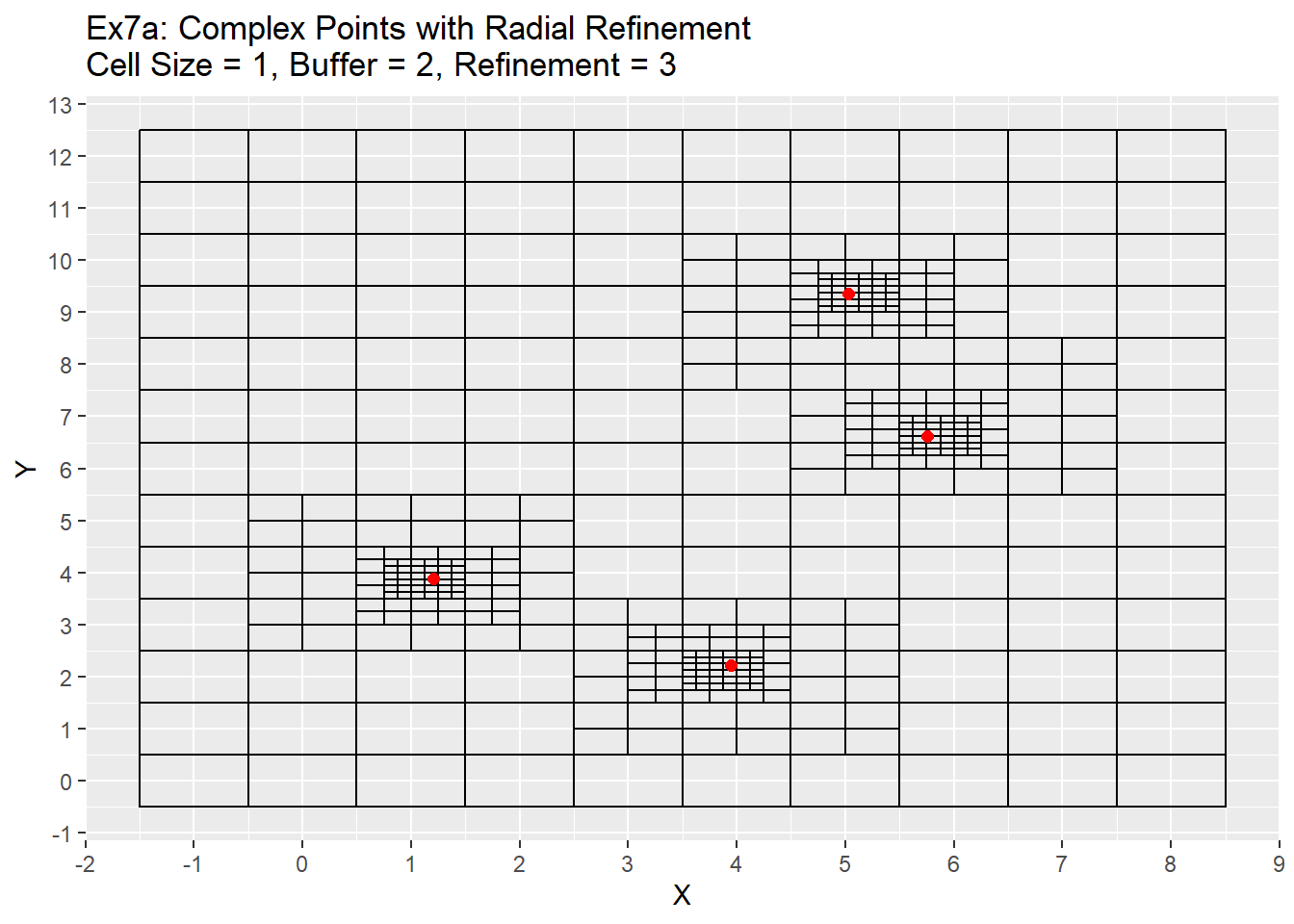
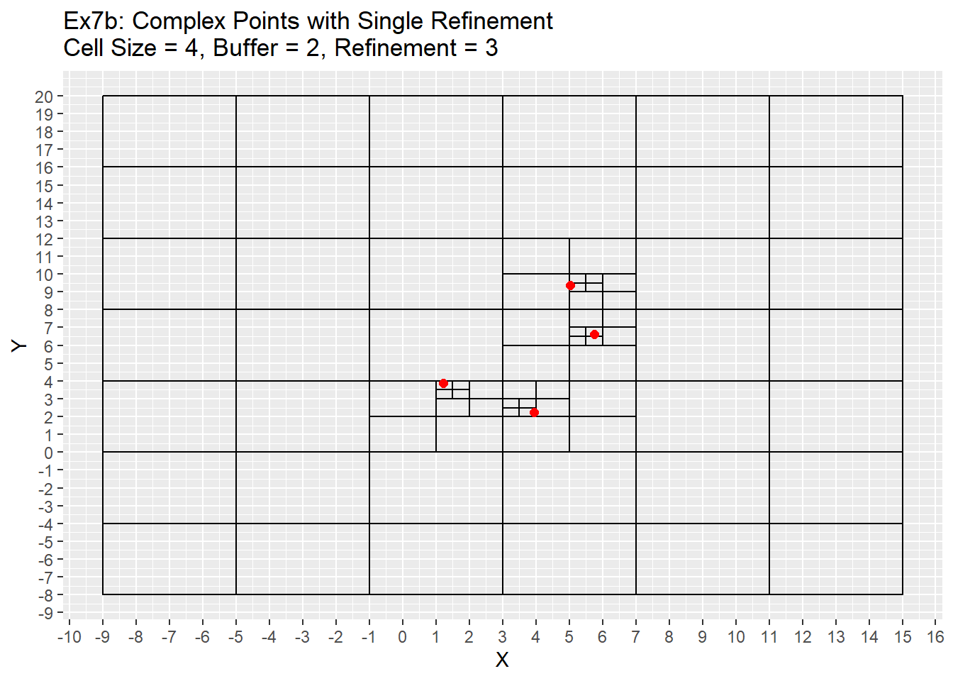
For our final example I will be revisiting example 3c from earlier. I have reran it using the main function and with three level refinement process. From the graph it is apparent that now all the points are located within their own unique cell, while still retaining the larger cell size. This allows for individual points to be allocated to a unique cell while also maintaining a larger grid size around those points.
Ex6_Grid <- Grid_Refinement_Function(x_coords = complex_points$X, y_coords = complex_points$Y, cell_size = 4, buffer = 2, num_ref = 3, ref_method = 'Single')

Ex6_Grid
##         x     y cell_size cell_id
##  1: -7.00 -6.00       4.0       1
##  2: -7.00 -2.00       4.0       2
##  3: -7.00  2.00       4.0       3
##  4: -7.00  6.00       4.0       4
##  5: -7.00 10.00       4.0       5
##  6: -7.00 14.00       4.0       6
##  7: -7.00 18.00       4.0       7
##  8: -3.00 -6.00       4.0       8
##  9: -3.00 -2.00       4.0       9
## 10: -3.00  2.00       4.0      10
## 11: -3.00  6.00       4.0      11
## 12: -3.00 10.00       4.0      12
## 13: -3.00 14.00       4.0      13
## 14: -3.00 18.00       4.0      14
## 15:  0.00  1.00       2.0      15
## 16:  0.00  3.00       2.0      16
## 17:  1.00 -6.00       4.0      17
## 18:  1.00 -2.00       4.0      18
## 19:  1.00  6.00       4.0      19
## 20:  1.00 10.00       4.0      20
## 21:  1.00 14.00       4.0      21
## 22:  1.00 18.00       4.0      22
## 23:  1.25  3.25       0.5      23
## 24:  1.25  3.75       0.5      24
## 25:  1.50  2.50       1.0      25
## 26:  1.75  3.25       0.5      26
## 27:  1.75  3.75       0.5      27
## 28:  2.00  1.00       2.0      28
## 29:  2.50  2.50       1.0      29
## 30:  2.50  3.50       1.0      30
## 31:  3.25  2.25       0.5      31
## 32:  3.25  2.75       0.5      32
## 33:  3.50  3.50       1.0      33
## 34:  3.75  2.25       0.5      34
## 35:  3.75  2.75       0.5      35
## 36:  4.00  1.00       2.0      36
## 37:  4.00  5.00       2.0      37
## 38:  4.00  7.00       2.0      38
## 39:  4.00  9.00       2.0      39
## 40:  4.00 11.00       2.0      40
## 41:  4.50  2.50       1.0      41
## 42:  4.50  3.50       1.0      42
## 43:  5.00 -6.00       4.0      43
## 44:  5.00 -2.00       4.0      44
## 45:  5.00 14.00       4.0      45
## 46:  5.00 18.00       4.0      46
## 47:  5.25  6.25       0.5      47
## 48:  5.25  6.75       0.5      48
## 49:  5.25  9.25       0.5      49
## 50:  5.25  9.75       0.5      50
## 51:  5.50  7.50       1.0      51
## 52:  5.50  8.50       1.0      52
## 53:  5.75  6.25       0.5      53
## 54:  5.75  6.75       0.5      54
## 55:  5.75  9.25       0.5      55
## 56:  5.75  9.75       0.5      56
## 57:  6.00  1.00       2.0      57
## 58:  6.00  3.00       2.0      58
## 59:  6.00  5.00       2.0      59
## 60:  6.00 11.00       2.0      60
## 61:  6.50  6.50       1.0      61
## 62:  6.50  7.50       1.0      62
## 63:  6.50  8.50       1.0      63
## 64:  6.50  9.50       1.0      64
## 65:  9.00 -6.00       4.0      65
## 66:  9.00 -2.00       4.0      66
## 67:  9.00  2.00       4.0      67
## 68:  9.00  6.00       4.0      68
## 69:  9.00 10.00       4.0      69
## 70:  9.00 14.00       4.0      70
## 71:  9.00 18.00       4.0      71
## 72: 13.00 -6.00       4.0      72
## 73: 13.00 -2.00       4.0      73
## 74: 13.00  2.00       4.0      74
## 75: 13.00  6.00       4.0      75
## 76: 13.00 10.00       4.0      76
## 77: 13.00 14.00       4.0      77
## 78: 13.00 18.00       4.0      78
##         x     y cell_size cell_id
ggplot() +
  geom_rect(data = Ex6_Grid, aes(xmin = x - cell_size/2, ymin = y - cell_size/2, xmax = x + cell_size/2, ymax = y + cell_size/2), color = 'black', fill = NA) +
  geom_point(data = complex_points, aes(x = X, y = Y), color = 'red', size = 2) +
  labs(title = 'Ex7b: Complex Points with Single Refinement\nCell Size = 4, Buffer = 2, Refinement = 3') +
  scale_x_continuous(breaks = seq(-20,20,1)) +
  scale_y_continuous(breaks = seq(-20,20,1))
Future Plans
I plan to follow this post up with another post detailing a more real world example, and potentially adding in an additional function that will allow for the grid table output to be converted into a spatial polygon dataset.